
Step-by-Step Guide to Using the Principal Stress Formula
Understanding stress distribution within a material subjected to external loads is crucial in mechanical engineering design. Specifically, the principal stresses represent the maximum and minimum normal stresses acting at a point, providing critical information for predicting material failure. This comprehensive guide provides a step-by-step approach to using the principal stress formula, targeting engineering students, practicing engineers, and researchers seeking a reliable reference. We’ll cover the fundamental concepts, the formulas themselves, and real-world applications, along with worked examples to solidify your understanding.
Understanding Stress: A Foundation
Before delving into the principal stress formula, let's briefly review the basics of stress. Stress is defined as the force acting per unit area within a material. It can be normal stress (σ), which is perpendicular to the area, or shear stress (τ), which is parallel to the area. Normal stress can be tensile (positive) or compressive (negative).
Normal Stress (σ): Arises from forces pulling or pushing directly on the area. For example, applying a tensile load to a bar induces tensile normal stress: σ = F/A, where F is the applied force and A is the cross-sectional area. Shear Stress (τ): Arises from forces acting tangentially to the area. An example is shear stress in a bolt connecting two plates subjected to a tensile load.
In most real-world scenarios, a component experiences stress in multiple directions. Therefore, understanding the stress state at a point requires considering all the stress components acting on that point. This is where the concept of principal stresses becomes invaluable.
Defining Principal Stresses and Principal Planes
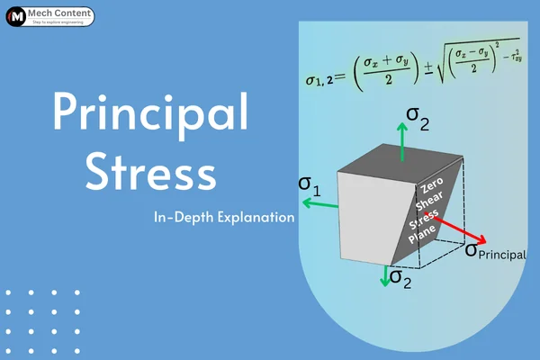
Principal stresses, denoted as σ1 and σ2 (in 2D) or σ1, σ2, and σ3 (in 3D), are the maximum and minimum normal stresses acting at a point. Importantly, at the planes where principal stresses act (called principal planes), the shear stress is zero. This simplifies the analysis because we're dealing with purely normal stresses, making it easier to predict failure using criteria like the maximum normal stress theory.
The orientation of these principal planes is crucial. Knowing the angle at which the maximum and minimum normal stresses occur allows engineers to align components or reinforce specific areas to better withstand the applied loads.
The Principal Stress Formula in Two Dimensions (Plane Stress)
The most common scenario encountered in introductory stress analysis is plane stress, where one dimension has negligible stress (e.g., a thin plate loaded in its plane). In this case, we have only two principal stresses to calculate. The principal stress formulas for the 2D (plane stress) state are:
σ1, σ2 = (σx + σy)/2 ± √[((σx - σy)/2)2 + τxy2]
Where: σ1 is the maximum principal stress. σ2 is the minimum principal stress. σx is the normal stress in the x-direction. σy is the normal stress in the y-direction. τxy is the shear stress acting on the x-y plane.
The angle θp that the principal plane makes with the x-axis is given by:
tan(2θp) = 2τxy / (σx - σy)
This equation yields two values for θp, differing by 90 degrees, representing the orientations of the two principal planes. We can then substitute these values back into the stress transformation equations to confirm which principal stress (σ1 or σ2) corresponds to each angle.
Step-by-Step Guide to Using the 2D Principal Stress Formula
Here's a detailed guide to calculating principal stresses and their orientations in 2D:
1.Determine the Stress State: Identify the normal stresses (σx and σy) and the shear stress (τxy) at the point of interest. Remember to use consistent sign conventions (tensile is positive, compressive is negative, and define a positive shear direction).
2.Calculate the Principal Stresses: Plug the values of σx, σy, and τxy into the principal stress formula: σ1, σ2 = (σx + σy)/2 ± √[((σx - σy)/2)2 + τxy2]. Calculate both σ1 and σ2, ensuring σ1 is the algebraically larger value.
3.Calculate the Principal Angle: Use the formula tan(2θp) = 2τxy / (σx - σy) to find the angle θp. Calculate 2θp first, then divide by 2 to obtain θp. Be mindful that the arctangent function (tan-1) typically returns a value between -90° and +90°. You may need to add or subtract 180° to one of the solutions to obtain the correct angles representing both principal planes.
4.Determine the Orientation of σ1 and σ2: To confirm which principal stress corresponds to which angle, substitute each θp value back into the stress transformation equations: σx' = (σx + σy)/2 + ((σx - σy)/2)cos(2θ) + τxysin(2θ)
τx'y' = -((σx - σy)/2)sin(2θ) + τxycos(2θ)
For each θp, calculate σx'. If σx' equals σ1, then that θp corresponds to σ1; otherwise, it corresponds to σ2. Also, τx'y' should be very close to zero for both principal planes.
5.Interpret the Results: The values of σ1 and σ2 represent the maximum and minimum normal stresses at the point, and the angles θp indicate the orientation of the planes on which these stresses act. This information is critical for predicting failure and optimizing the design.
Worked Example (2D)
Consider a point in a steel plate subjected to the following stresses: σx = 80 MPa, σy = -50 MPa, and τxy = 30 MPa. Determine the principal stresses and their orientations.
1.Stress State: σx = 80 MPa, σy = -50 MPa, τxy = 30 MPa.
2.Principal Stresses:
σ1, σ2 = (80 - 50)/2 ± √[((80 + 50)/2)2 + 302]
σ1, σ2 = 15 ± √[(65)2 + 302]
σ1, σ2 = 15 ± √(4225 + 900)
σ1, σ2 = 15 ± √5125
σ1, σ2 = 15 ± 71.59
σ1 = 15 + 71.59 =
86.59 MPa
σ2 = 15 - 71.59 = -56.59 MPa
3.Principal Angle:
tan(2θp) = 2(30) / (80 - (-50)) = 60 / 130 = 0.4615
2θp = tan-1(0.4615) =
24.77°
θp1 = 24.77° / 2 =
12.39°
Since tan(x) = tan(x + 180°), we have a second solution:
2θp2 = 24.77° + 180° =
204.77°
θp2 = 204.77° / 2 =
102.39°
4.Orientation of σ1 and σ2:
Using θp1 = 12.39° in the stress transformation equation:
σx' = (80 - 50)/2 + ((80 + 50)/2)cos(212.39°) + 30sin(212.39°)
σx' = 15 + (65)cos(24.78°) + 30sin(24.78°)
σx' = 15 + 59.05 +
12.59 =
86.64 MPa ≈ σ1
Therefore, σ1 = 86.59 MPa acts on the plane oriented at
12.39° relative to the x-axis. Consequently, σ2 = -56.59 MPa acts on the plane oriented at
102.39° relative to the x-axis.
5.Interpretation: The maximum tensile stress at the point is
86.59 MPa, acting on a plane rotated
12.39° from the x-axis. The minimum stress is -56.59 MPa (compressive), acting on a plane rotated
102.39° from the x-axis.
Principal Stress in Three Dimensions
The principal stress calculation in 3D is more complex and involves finding the eigenvalues of the stress tensor. The stress tensor is a 3x3 matrix that represents the stress state at a point:
[σx τxy τxz]
[τyx σy τyz]
[τzx τzy σz]
Where τxy = τyx, τxz = τzx, and τyz = τzy.
The principal stresses (σ1, σ2, σ3) are the roots of the characteristic equation:
det(σ - σI) = 0
Where: σ is the stress tensor. σ is a variable representing the principal stress values. I is the identity matrix.
det() denotes the determinant of the matrix.
Expanding the determinant results in a cubic equation in σ. Solving this cubic equation gives the three principal stresses. While analytical solutions exist for cubic equations, numerical methods are often employed in practice, especially when dealing with complex stress states. Software packages like ANSYS, Abaqus, and COMSOL are typically used to perform 3D stress analysis and calculate principal stresses.
When should principal stress formulas be applied in design?
Principal stress calculations are essential when designing components subjected to multiaxial loading. They help determine the maximum tensile and compressive stresses, crucial for predicting failure according to various failure theories such as the maximum normal stress theory, the maximum shear stress theory (Tresca criterion), and the distortion energy theory (von Mises criterion).
How do you calculate hoop stress in thin-walled cylinders?
Hoop stress (σh) in a thin-walled cylinder subjected to internal pressure (p) is calculated using the formula σh = (pr)/t, where 'r' is the radius of the cylinder and 't' is the wall thickness. This formula directly relates to principal stress as the hoop stress is a principal stress in the circumferential direction. The axial stress (σa) is another principal stress and is given by σa = (pr)/(2t).
What is the difference between true stress and engineering stress?
Engineering stress is calculated by dividing the applied force by theoriginalcross-sectional area of the material (σe = F/A0). True stress, on the other hand, is calculated by dividing the applied force by theinstantaneouscross-sectional area of the material (σt = F/Ai). True stress provides a more accurate representation of the stress experienced by the material during deformation, especially at large strains. For small deformations, the difference between the two is negligible, but as the material necks or undergoes significant changes in cross-section, the true stress becomes significantly higher than the engineering stress. Principal stresses are typically calculated using engineering stress values, but in situations involving large deformations, true stress values should be considered.
Real-World Applications
Principal stress analysis finds applications in various engineering fields: Pressure Vessels: Determining the maximum stress in pressure vessel walls to prevent rupture. The hoop stress and axial stress are principal stresses in this case. Beams: Calculating the maximum tensile and compressive stresses in beams under bending to ensure they don't yield or fracture. Rotating Machinery: Analyzing stresses in rotating components like turbine blades and shafts to prevent fatigue failure. Structural Analysis: Assessing the stress distribution in buildings and bridges to ensure structural integrity under various load conditions. Thermal Stress:Evaluating stresses induced by temperature gradients in components subjected to heating or cooling.
Common Pitfalls and Misconceptions
Incorrect Sign Conventions: Consistent sign conventions are crucial. Ensure tensile stress is positive and compressive stress is negative. Similarly, define a consistent positive direction for shear stress. Ignoring Shear Stress: In some simplified analyses, shear stress is neglected. However, it's crucial to include shear stress in the principal stress calculation when it's significant. Applying 2D Formulas to 3D Problems: The 2D principal stress formula is only valid for plane stress conditions. Using it for 3D problems will lead to inaccurate results. Misinterpreting Principal Angles: The principal angles represent theorientationof the planes on which the principal stresses act, not the magnitude of the stresses themselves.
Conclusion
The principal stress formula is a powerful tool for analyzing stress states and predicting material failure. By understanding the underlying concepts and following the step-by-step guide provided, engineers can confidently calculate principal stresses and use this information to design safer and more efficient structures and machines. Remember to consider the limitations of the 2D and 3D formulas, and always verify your results using appropriate software tools when dealing with complex geometries and loading conditions.